Protect several linked tables at once

Introduction

In rtauargus package, it is now possible to protect a set of linked tables at once. The function to do this is called tab_multi_manager(). The very simple algorithm implemented to handle the protection doesn’t depend on the number of tables. Hence, the function can theoretically deal with an indefinite number of tables. Of course, the practical use is limited by the power of the computer. However, we are confident on the ability of the function to treat the most cases. We are interested in cases that you would encounter and the function can’t handle.

A link between two (or more) tables describes the common cells of the tables, that is the cells appearing in them. The function can handle all types of links between tables:

margin links: when two tables share one (or more) variables;
links between the response variables, when exists some equations connecting the variables;
non-nested hierarchies: when an explanatory variable is broken down into two (or more) non-nested hierarchies.

Actually, the last two types can be handled as the first one. The challenge for the user is to properly define the set of the tables. Once the set is correctly defined, the function takes care of everything.

Firstly, the vignette will present how the function works, secondly, the parameters are quickly described. In the third part, some examples are developped to show how to use it in diverse situations.

How does `tab_multi_manager()` handle the protection of a set of linked tables ?

Firstly, the function merges all the tables of the set. In the resulted table, boolean variables are added to mention whether a cell owns to a given table of the set. So, there are as many boolean variables as the number of tables in the set. The merged table is a very effective way to quickly detect the common cells. Thus, the report of the suppressions is automatic.

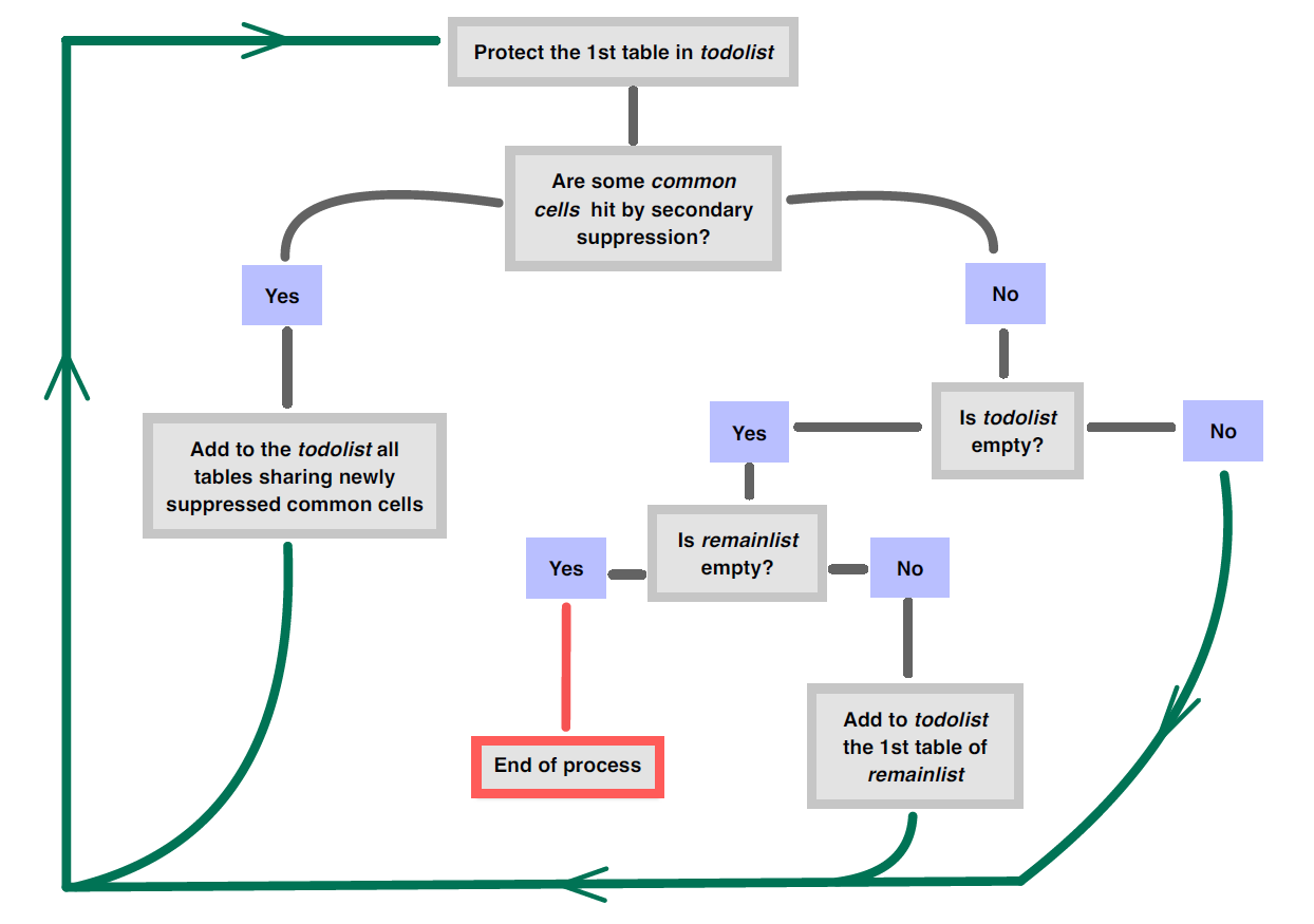
The protection process is sequential: one table at a time. To handle the protection of all the tables and not to forget one table or some links, the implemented algorithm works with two lists:

todolist: list of tables which have to be protected;
remainlist: list of original tables which haven’t yet been protected at all.

Both lists are initialized as follows:

todolist = first table in the original list;
remainlist = all the original tables except the firs one.

Then, the algorithm proceeds as shown in the following figure:

How tab_multi_manager's algorithm works

Results

The function returns the original list of tables with some other variables which are boolean variables (TRUE if the cell has to be masked, otherwise FALSE), describing all steps of the suppression process. Each step takes the previous one into account and the last variable indicates the final step. Final status of cell is easily computable with this last variable and the primary suppression status previously computed by the user.

In addition, the function writes all τ-Argus files created during the process. At the end, only the last process for each table is available in the chosen directory. A journal (journal.txt) is also provided. It describes each step of the suppression process: Which table is being protected, how many new common cells have been hit by secondary suppression. At the end of the process, it provides a description of all common cells that have been hit, mentionning the iteration of when each has been hit.

Some details on the parameters of `tab_multi_manager()`

dir_name the directory that will contain all the created files, if non existing it will be created. example : dir_name = “my_directory”
hrc A named vector specifying the path to the hrc file for each hierarchical variables. example : c(ACTIVITY = “path_to_file/act.hrc”, NUTS = “path_to_file/nuts.hrc” )
alt_hrc A named list useful for dealing with non-nested hierachies. The names of the list are the names of the tables when alternative (non-nested in general) hierarchies. example : If T1 and T2 have one explanatory variable, called ACTIVITY, and the same response variable, but the ACTIVITY variable has not the same hierarchy in the two tables. Let’s assume that the hierarchies (act1.hrc and act2.hrc) are not nested. In that case, we write the two arguments as follows:
- hrc = c(ACTIVITY = “path_to_file/act_1.hrc”): By default, this hierarchy will be used.
- alt_hrc = list(T2 = c(ACTIVITY = “path_to_file/act_2.hrc”)): In the table T2, the alternative hierarchy will be used.
totcode The code for total for each explanatory variables. It is recommanded to use the same totcode for each variables. If for example the code is “Total” for all variables. This syntax is allowed : totcode = “Total”

Otherwise the expected input is a list specifying the totcode for each explanatory vars. For example : totcode = list(ACTIVITY = “Total”, NUTS = “FR”, SIZE =“Ensemble”, CJ = “Total”) Default : “Total”

Warning : If the totals are not in the table, they will be computed by Tau-Argus, but they won’t be eligible for primary suppression. We, then, advise users to provide totals in their tables.

alt_totcode A named list for alternative total codes. See alt_hrc for use.
value The colname of the response variable in the tables, it MUST be the same name for each tables. For example : value = “turnover” Default : “value”
freq The colname of the frequency variable in the tables, it MUST be the same name for each tables. For example : freq = “frequency” Default : “freq”
secret_var The name of the boolean variable specifying primary suppression in the tables, it MUST be the same name for each tables. For example : secret_var = “is_secret_prim” Default : “is_secret_prim”
suppress The algorithm required to perform secondary suppression, explained in the safety_rules vignette. If Modular approach is chosen, after the first iteration on a given table, the singleton, multi-singleton and minFreq options are deactivated. default : MOD(1,5,1,0,0)”
ip_start The manual safety range for the first iteration on a table (integer) default : 10
ip_end The manual safety range for the second iteration on a table (integer) default : 0
num_iter_max This parameter is here to ensure the fact that the function will stop. default : 10

Some examples

Let’s specify the location of the TauArgus.exe file in our computer:

options(
  rtauargus.tauargus_exe =
    "Y:/Logiciels/TauArgus/TauArgus4.2.3/TauArgus.exe"
)

About protecting 4 linked tables at once

In the following example we are going to protect a set of 4 linked tables sharing the same response variable, that is turnover.

Preparing the data

data("turnover_act_size")
data("turnover_act_cj")
data ("turnover_nuts_size")
data("turnover_nuts_cj")

ACTIVITY X SIZE named turnover_act_size ACTIVITY X CJ named turnover_act_cj NUTS X SIZE named turnover_nuts_size NUTS X CJ named turnover_nuts_cj

str(turnover_act_size)
#> tibble [414 x 5] (S3: tbl_df/tbl/data.frame)
#>  $ ACTIVITY: chr [1:414] "AZ" "BE" "FZ" "GI" ...
#>  $ SIZE    : chr [1:414] "Total" "Total" "Total" "Total" ...
#>  $ N_OBS   : int [1:414] 405 12878 28043 62053 8135 8140 11961 41359 26686 25108 ...
#>  $ TOT     : num [1:414] 44475 24827613 8907311 26962063 8584917 ...
#>  $ MAX     : num [1:414] 6212 1442029 1065833 3084242 3957364 ...
str(turnover_nuts_cj)
#> tibble [452 x 5] (S3: tbl_df/tbl/data.frame)
#>  $ NUTS : chr [1:452] "FR10" "FR21" "FR22" "FR23" ...
#>  $ CJ   : chr [1:452] "Total" "Total" "Total" "Total" ...
#>  $ N_OBS: int [1:452] 38462 6769 4561 5090 8611 7811 5643 10411 8179 5163 ...
#>  $ TOT  : num [1:452] 33026385 2947560 1917663 3701935 5089279 ...
#>  $ MAX  : num [1:452] 3084242 544763 651848 298134 1165019 ...

The first step is to create a list containing our four tables, it is advised to give a name to each tables. By doing so it will be easier to track secondary suppression.

list_data_4_tabs <- list(
  act_size = turnover_act_size,
  act_cj = turnover_act_cj,
  nuts_size = turnover_nuts_size,
  nuts_cj = turnover_nuts_cj
)
str(list_data_4_tabs)
#> List of 4
#>  $ act_size : tibble [414 x 5] (S3: tbl_df/tbl/data.frame)
#>   ..$ ACTIVITY: chr [1:414] "AZ" "BE" "FZ" "GI" ...
#>   ..$ SIZE    : chr [1:414] "Total" "Total" "Total" "Total" ...
#>   ..$ N_OBS   : int [1:414] 405 12878 28043 62053 8135 8140 11961 41359 26686 25108 ...
#>   ..$ TOT     : num [1:414] 44475 24827613 8907311 26962063 8584917 ...
#>   ..$ MAX     : num [1:414] 6212 1442029 1065833 3084242 3957364 ...
#>  $ act_cj   : tibble [406 x 5] (S3: tbl_df/tbl/data.frame)
#>   ..$ ACTIVITY: chr [1:406] "AZ" "BE" "FZ" "GI" ...
#>   ..$ CJ      : chr [1:406] "Total" "Total" "Total" "Total" ...
#>   ..$ N_OBS   : int [1:406] 405 12878 28043 62053 8135 8140 11961 41359 26686 25108 ...
#>   ..$ TOT     : num [1:406] 44475 24827613 8907311 26962063 8584917 ...
#>   ..$ MAX     : num [1:406] 6212 1442029 1065833 3084242 3957364 ...
#>  $ nuts_size: tibble [460 x 5] (S3: tbl_df/tbl/data.frame)
#>   ..$ NUTS : chr [1:460] "FR10" "FR21" "FR22" "FR23" ...
#>   ..$ SIZE : chr [1:460] "Total" "Total" "Total" "Total" ...
#>   ..$ N_OBS: int [1:460] 38462 6769 4561 5090 8611 7811 5643 10411 8179 5163 ...
#>   ..$ TOT  : num [1:460] 33026385 2947560 1917663 3701935 5089279 ...
#>   ..$ MAX  : num [1:460] 3084242 544763 651848 298134 1165019 ...
#>  $ nuts_cj  : tibble [452 x 5] (S3: tbl_df/tbl/data.frame)
#>   ..$ NUTS : chr [1:452] "FR10" "FR21" "FR22" "FR23" ...
#>   ..$ CJ   : chr [1:452] "Total" "Total" "Total" "Total" ...
#>   ..$ N_OBS: int [1:452] 38462 6769 4561 5090 8611 7811 5643 10411 8179 5163 ...
#>   ..$ TOT  : num [1:452] 33026385 2947560 1917663 3701935 5089279 ...
#>   ..$ MAX  : num [1:452] 3084242 544763 651848 298134 1165019 ...

Applying primary suppression rules

Then we need to apply the primary suppression for each table. Here we apply 2 rules : The dominance rule NK(1,85) and the frequency rule with a threshold set to 3.

list_data_4_tabs <- list_data_4_tabs %>%
  purrr::map(
    function(df){
      df %>%
        mutate(
          is_secret_freq = N_OBS > 0 & N_OBS < 3,
          is_secret_dom = ifelse(MAX == 0, FALSE, MAX/TOT>0.85),
          is_secret_prim = is_secret_freq | is_secret_dom
        )
    }
  )
str(list_data_4_tabs)
#> List of 4
#>  $ act_size : tibble [414 x 8] (S3: tbl_df/tbl/data.frame)
#>   ..$ ACTIVITY      : chr [1:414] "AZ" "BE" "FZ" "GI" ...
#>   ..$ SIZE          : chr [1:414] "Total" "Total" "Total" "Total" ...
#>   ..$ N_OBS         : int [1:414] 405 12878 28043 62053 8135 8140 11961 41359 26686 25108 ...
#>   ..$ TOT           : num [1:414] 44475 24827613 8907311 26962063 8584917 ...
#>   ..$ MAX           : num [1:414] 6212 1442029 1065833 3084242 3957364 ...
#>   ..$ is_secret_freq: logi [1:414] FALSE FALSE FALSE FALSE FALSE FALSE ...
#>   ..$ is_secret_dom : logi [1:414] FALSE FALSE FALSE FALSE FALSE FALSE ...
#>   ..$ is_secret_prim: logi [1:414] FALSE FALSE FALSE FALSE FALSE FALSE ...
#>  $ act_cj   : tibble [406 x 8] (S3: tbl_df/tbl/data.frame)
#>   ..$ ACTIVITY      : chr [1:406] "AZ" "BE" "FZ" "GI" ...
#>   ..$ CJ            : chr [1:406] "Total" "Total" "Total" "Total" ...
#>   ..$ N_OBS         : int [1:406] 405 12878 28043 62053 8135 8140 11961 41359 26686 25108 ...
#>   ..$ TOT           : num [1:406] 44475 24827613 8907311 26962063 8584917 ...
#>   ..$ MAX           : num [1:406] 6212 1442029 1065833 3084242 3957364 ...
#>   ..$ is_secret_freq: logi [1:406] FALSE FALSE FALSE FALSE FALSE FALSE ...
#>   ..$ is_secret_dom : logi [1:406] FALSE FALSE FALSE FALSE FALSE FALSE ...
#>   ..$ is_secret_prim: logi [1:406] FALSE FALSE FALSE FALSE FALSE FALSE ...
#>  $ nuts_size: tibble [460 x 8] (S3: tbl_df/tbl/data.frame)
#>   ..$ NUTS          : chr [1:460] "FR10" "FR21" "FR22" "FR23" ...
#>   ..$ SIZE          : chr [1:460] "Total" "Total" "Total" "Total" ...
#>   ..$ N_OBS         : int [1:460] 38462 6769 4561 5090 8611 7811 5643 10411 8179 5163 ...
#>   ..$ TOT           : num [1:460] 33026385 2947560 1917663 3701935 5089279 ...
#>   ..$ MAX           : num [1:460] 3084242 544763 651848 298134 1165019 ...
#>   ..$ is_secret_freq: logi [1:460] FALSE FALSE FALSE FALSE FALSE FALSE ...
#>   ..$ is_secret_dom : logi [1:460] FALSE FALSE FALSE FALSE FALSE FALSE ...
#>   ..$ is_secret_prim: logi [1:460] FALSE FALSE FALSE FALSE FALSE FALSE ...
#>  $ nuts_cj  : tibble [452 x 8] (S3: tbl_df/tbl/data.frame)
#>   ..$ NUTS          : chr [1:452] "FR10" "FR21" "FR22" "FR23" ...
#>   ..$ CJ            : chr [1:452] "Total" "Total" "Total" "Total" ...
#>   ..$ N_OBS         : int [1:452] 38462 6769 4561 5090 8611 7811 5643 10411 8179 5163 ...
#>   ..$ TOT           : num [1:452] 33026385 2947560 1917663 3701935 5089279 ...
#>   ..$ MAX           : num [1:452] 3084242 544763 651848 298134 1165019 ...
#>   ..$ is_secret_freq: logi [1:452] FALSE FALSE FALSE FALSE FALSE FALSE ...
#>   ..$ is_secret_dom : logi [1:452] FALSE FALSE FALSE FALSE FALSE FALSE ...
#>   ..$ is_secret_prim: logi [1:452] FALSE FALSE FALSE FALSE FALSE FALSE ...

Three variables have been added to each table. Only the last one will be used during the protection process. The two others will be useful to state the final status of the cells.

Preparing the list of explanatory variables

Then we are going to create the list of explanatory variables of the tables. In our case, the explanatory variables are the 2 first columns of each table.

nom_var_list <- purrr::map(
  list_data_4_tabs,
  function(data) colnames(data)[1:2]
)
nom_var_list
#> $act_size
#> [1] "ACTIVITY" "SIZE"    
#> 
#> $act_cj
#> [1] "ACTIVITY" "CJ"      
#> 
#> $nuts_size
#> [1] "NUTS" "SIZE"
#> 
#> $nuts_cj
#> [1] "NUTS" "CJ"

The names of the list have to be the names of the corresponding tables in the list_tables argument.

Preparing the list of total codes

The labels used to mention the total for each variable have to declared by the user, in a named list. However, when all of the variables have the same label to refer to the total, the information can be mentionned as follows:

total_codes <- "Total"

Making the hierarchical files

ACTIVITY and NUTS are two hierarchical variables. We use a correspondance table for each of them to create the .hrc files that tau-Argus need.

data(activity_corr_table)
data(nuts23_fr_corr_table)

hrc_file_activity <- write_hrc2(
  corr_table = activity_corr_table,
  file_name = "hrc/activity.hrc"
)
hrc_file_nuts <- write_hrc2(
  corr_table = nuts23_fr_corr_table,
  file_name = "hrc/nuts.hrc"
)

To mention the names of the hrc files, we create a named vector (or list) as follows:

hrc_files <- list(
  ACTIVITY = hrc_file_activity,
  NUTS = hrc_file_nuts
)

The names of the vector have to be the names of the corresponding hierarchical variables.

Running the protection of all the tables at once

res <- tab_multi_manager(
    list_tables = list_data_4_tabs,
    list_explanatory_vars = nom_var_list,
    dir_name = "tauargus_files/ex4",
    hrc = hrc_files,
    totcode = total_codes,
    value = "TOT",
    freq = "N_OBS",
    secret_var = "is_secret_prim"
)
#> --- Current table to treat:  act_size ---
#> --- Current table to treat:  act_cj ---
#> --- Current table to treat:  act_size ---
#> --- Current table to treat:  nuts_size ---
#> --- Current table to treat:  nuts_cj ---

Results

list_with_status <- res %>%
  purrr::map(
    function(df){
      df %>%
        rename_with(~"final_suppress", last_col()) %>%
        mutate(
          status = case_when(
            is_secret_freq ~ "A",
            is_secret_dom ~ "B",
            final_suppress ~ "D",
            TRUE ~"V"
          )
        ) %>%
        select(1:2, TOT, N_OBS, status)
    }
  )
str(list_with_status$act_size)
#> 'data.frame':    414 obs. of  5 variables:
#>  $ ACTIVITY: chr  "01" "01" "02" "02" ...
#>  $ SIZE    : chr  "Total" "tr1" "Total" "tr1" ...
#>  $ TOT     : num  853 853 43623 35503 8120 ...
#>  $ N_OBS   : int  18 18 387 381 6 1 1 4 4 84 ...
#>  $ status  : chr  "V" "V" "V" "V" ...

list_with_status %>%
  purrr::iwalk(
    function(df,name){
      cat(name, "\n")
      df %>% count(status) %>% print()
    }
  )
#> act_size 
#>   status   n
#> 1      A  52
#> 2      B  25
#> 3      D  83
#> 4      V 254
#> act_cj 
#>   status   n
#> 1      A  35
#> 2      B  25
#> 3      D  88
#> 4      V 258
#> nuts_size 
#>   status   n
#> 1      A  55
#> 2      B  17
#> 3      D  82
#> 4      V 306
#> nuts_cj 
#>   status   n
#> 1      A  45
#> 2      B  20
#> 3      D 101
#> 4      V 286

Dealing with non-nested hierarchies

Let’s assume that we’d like to protect the two tables crossing ACTIVITY and SIZE in one hand and ACTIVITY and CJ in the other hand. The ACTIVITY variable is a hierarchical one. Moreover, in that case, we’d like to release a subtotal, called D_TO_M, in addition to those in the activity_corr_table. This subtotal is the sum of the D to M labels of the A21 level. As this subtotal can’t be inserted in the main hierarchy, this leads us to a case of non-nested hierarchies.

To confirm the non-nesting of the two hierachies, let’s display an extract of both.

Extract of the main hierarchy:

sdcHierarchies::hier_create(
  root="Total",
  nodes = activity_corr_table$A10 %>% unique()
) %>%
  sdcHierarchies::hier_display()
#> Total
#> +-AZ
#> +-BE
#> +-FZ
#> +-GI
#> +-JZ
#> +-KZ
#> +-LZ
#> +-MN
#> +-OQ
#> \-RU

Extract of the alternative hierarchy:

sdcHierarchies::hier_create(
  root="D_TO_M",
  nodes = activity_corr_table_D_TO_M$A21
) %>%
  sdcHierarchies::hier_display()
#> Error in sdcHierarchies::hier_create(root = "D_TO_M", nodes = activity_corr_table_D_TO_M$A21): object 'activity_corr_table_D_TO_M' not found

To handle this case, the preferred approach is to create a third table crossing ACTIVITY and SIZE with D to M labels and the subtotal D_TO_M:

turnover_act_size_D_TO_M <- turnover_act_size %>%
  filter(
    ACTIVITY %in% LETTERS[4:13]
  ) %>%
  bind_rows(
    turnover_act_size %>%
      filter(
        ACTIVITY %in% LETTERS[4:13]
      ) %>%
      group_by(SIZE) %>%
      summarise(N_OBS = sum(N_OBS), TOT = sum(TOT), MAX = max(MAX)) %>%
      mutate(ACTIVITY = "D_TO_M")
  )
str(turnover_act_size_D_TO_M)
#> tibble [44 x 5] (S3: tbl_df/tbl/data.frame)
#>  $ ACTIVITY: chr [1:44] "D" "E" "F" "G" ...
#>  $ SIZE    : chr [1:44] "Total" "Total" "Total" "Total" ...
#>  $ N_OBS   : int [1:44] 1411 828 28043 41624 6524 13905 8135 8140 11961 28221 ...
#>  $ TOT     : num [1:44] 2438454 2264393 8907311 18244309 6273334 ...
#>  $ MAX     : num [1:44] 981369 306905 1065833 765244 3084242 ...

Let’s create the alternative hierarchy file.

activity_corr_table_D_TO_M <- activity_corr_table %>%
  filter(A21 %in% LETTERS[4:13]) %>%
  select(-A88) %>%
  mutate(A10 = "D_TO_M") %>%
  unique()

hrc_file_activity_D_TO_M <- activity_corr_table_D_TO_M %>%
  select(-1) %>%
  write_hrc2(file_name = "hrc/activity_D_TO_M")

Then, let’s build the list of tables and apply the primary suppression rules on them.

list_data_3_tabs_nn <- list(
  act_size = turnover_act_size,
  act_size_D_TO_M = turnover_act_size_D_TO_M,
  act_cj = turnover_act_cj
) %>%
  purrr::map(
    function(df){
      df %>%
        mutate(
          is_secret_freq = N_OBS > 0 & N_OBS < 3,
          is_secret_dom = ifelse(MAX == 0, FALSE, MAX/TOT>0.85),
          is_secret_prim = is_secret_freq | is_secret_dom
        )
    }
  )

The hrc and alt_hrc arguments are used to mention both hierarchies of the ACTIVITY variable:

hrc is used as int the previous example (a named vector where names are the different hierarchical variables appearingin the tables and values are the files names). Hence, the hierarchy file will be taken in this vector by default.
alt_hrc is only used to mention the alternative hierarchies. This argument is a named list where names are the tables where the alternative hierarchies have to be applied.

The same rationale is used to fill the alt_totcode argument.

res <- tab_multi_manager(
  list_tables = list_data_3_tabs_nn,
  list_explanatory_vars = list(
    act_size = c("ACTIVITY", "SIZE"),
    act_size_D_TO_M = c("ACTIVITY", "SIZE"),
    act_cj = c("ACTIVITY", "CJ")
  ),
  hrc = c(ACTIVITY = hrc_file_activity),
  alt_hrc = list(
    act_size_D_TO_M = c(ACTIVITY = hrc_file_activity_D_TO_M)
  ),
  dir_name = "tauargus_files/ex5",
  value = "TOT",
  freq = "N_OBS",
  secret_var = "is_secret_prim",
  totcode =  "Total",
  alt_totcode = list(
    act_size_D_TO_M = c(ACTIVITY = "D_TO_M")
  )
)
#> --- Current table to treat:  act_size ---
#> --- Current table to treat:  act_size_D_TO_M ---
#> --- Current table to treat:  act_cj ---
#> --- Current table to treat:  act_size ---
#> --- Current table to treat:  act_size_D_TO_M ---
#> --- Current table to treat:  act_size ---
#> --- Current table to treat:  act_cj ---

About this vignette

Authors: Julien Jamme & Nathanael Rastout
Last update: 21/09/2023
Version of rtauargus used: 1.2.0
Version of τ-Argus used : TauArgus 4.2.3
R version used : 4.2.3

summary ↑

¶ Package {rtauargus} ¶

Introduction

How does tab_multi_manager() handle the protection of a set of linked tables ?

Results

Some details on the parameters of tab_multi_manager()

Some examples

About protecting 4 linked tables at once

Preparing the data

Applying primary suppression rules

Preparing the list of explanatory variables

Preparing the list of total codes

Making the hierarchical files

Running the protection of all the tables at once

Results

Dealing with non-nested hierarchies

About this vignette

¶
Package {rtauargus} ¶

How does `tab_multi_manager()` handle the protection of a set of linked tables ?

Some details on the parameters of `tab_multi_manager()`