Suppressive methods

For tabular data

INSEE, Department of Statistical Methods

Methods Available

Two types of methods depending on when they are applied:

• Pre-tabulation methods are applied to individual data, i.e. before any tabulation
• Post-tabulation methods are applied to aggregated data, i.e. after tabulation

Post-Tabulation Methods

Grouping of categories and removal of cells.

Frequency Tables

	North	West	East	South	Total
Polluting	6	14	1	7	28
Non-polluting	3	2	1	13	19
Total	9	16	2	20	47

Table 1: Number of polluting companies by region

Are there any cells at risk?

Staffing Tables

Frequency rule: a cell in a table must not be constructed from strictly fewer than n units (n > 0).

For data entered at the Insee, n = 3.

Staffing Tables

	Nord	Ouest	Est	Sud	Total
Polluting	6	14	1	7	28
Non-polluting	3	2	1	13	19
Total	9	16	2	20	47

Table 2: Number of polluting companies by region

Volume Tables

	Harpes	Piano	Orgues	Total
Nord	58	71	92	221
Centre	11	124	157	292
Sud	36	24	60	120
Total	105	219	309	633

Table 3: Distribution of instrument sales by region and by type, in millions of euros

Are there any cells at risk?

Volume Tables

Region	Harps	Piano	Organs	Total
North	58 (5)	71 (17)	92 (5)	221 (27)
Center	11 (4)	124 (11)	157 (2)	292 (17)
South	36 (3)	24 (6)	60 (1)	120 (10)
Total	105 (12)	219 (34)	309 (8)	633 (54)

Table 4: Distribution of instrument sales by region and type, in millions of euros

Note: the values in parentheses indicate the number of contributors.

Volume Tables

Primary frequency secret.

Region	Harps	Piano	Organs	Total
North	58 (5)	71 (17)	92 (5)	221 (27)
Center	11 (4)	124 (11)	157 (2)	292 (17)
South	36 (3)	24 (6)	60 (1)	120 (10)
Total	105 (12)	219 (34)	309 (8)	633 (54)

Table 5: Distribution of instrument sales by region and type, in millions of euros

Note: the values in parentheses indicate the number of contributors.

Volume Tables

Dominance Rule (n,k): a cell is sensitive if the n largest contributors to that cell represent more than k% of the cell’s total.

• For business data at INSEE, n = 1 and k = 85. Therefore, 1 contributing unit to a cell cannot contribute more than 85% of that cell’s value.
• For each cell in the table, it is necessary to determine the largest contributor.

Volume Tables

Primary dominance secret.

Region	Harps	Piano	Organs	Total
North	58 (5)	71 (17)	92 (5)	221 (27)
Center	11 (4)	124 (11)	157 (2)	292 (17)
South	36 (3)	24 (6)	60 (1)	120 (10)
Total	105 (12)	219 (34)	309 (8)	633 (54)

Table 6: Distribution of instrument sales by region and type, in millions of euros

Note: the values in parentheses indicate the number of contributors.

Volume Tables

p% Rule: a cell is sensitive if one of the contributors who has a cell can estimate the value of another contributor to p% of its true value.

• In practice, the 2nd contributor to the cell’s value must not be able to estimate, using their own value, that of the first contributor with a precision greater than p%.
• It is customary to choose p = 10.
• Not used at Insee but recommended by European experts.

Volume Tables

Primary secret due to the p% rule

Region	Harps	Piano	Organs	Total
North	58 (5)	71 (17)	92 (5)	221 (27)
Center	11 (4)	124 (11)	157 (2)	292 (17)
South	36 (3)	24 (6)	60 (1)	120 (10)
Total	105 (12)	219 (34)	309 (8)	633 (54)

Table 7: Distribution of instrument sales by region and type, in millions of euros

Note: the values in parentheses indicate the number of contributors.

The Primary Secret

Cells categorized as at risk for the frequency rule, the dominance rule, and the p% rule constitute the primary secret. These cells cannot be disseminated.

How to do it?

Category Grouping

Redefine the content of the crosstabulation variables by reducing the number of their modalities.

This strongly reduces, or even completely eliminates, primary secrecy.

Consider this option before other methods.

Recoding: An Example

	<25	25-30	30-50	> 50	Total
Polluting	2	5	7	6	20
Non-polluting	8	15	17	20	60
Total	10	20	24	26	80

Table 8: Number of polluting companies according to the age of the manager

Define new modalities to increase the number of respondents per cell.

Recoding: an example

	<28	28-35	35-55	> 55	Total
Polluting	3	6	6	5	20
Non-polluting	9	17	19	15	60
Total	12	23	25	20	80

Table 9: Number of polluting companies by age of manager

Recoding: Your Turn!

We aim to publish the following table:

• Population of a region by their department of residence, their department of work, their profession, and their age.
• A lot of primary secrecy in this table since most people reside and work in the same department.
• How to recode this table?

The first recoding consists of grouping all work departments outside the department of residence into a single category.

Recoding

👍	👎
Reduces the SP.	Does not always completely eliminate the SP.
Very simple to implement.	Impossible in some cases (imposed structure, longitudinal follow-up).

How to protect the remaining primary secret?

Cell Suppression

Primary Secret

First step: remove cells that do not comply with primary secret rules.

	North	West	East	South	Total
Polluting	6	14	X	7	28
Non-polluting	3	X	3	13	21
Total	9	16	4	20	49

Table 10: Number of polluting businesses by region

This is not sufficient; the cells are linked to each other by equations (margins).

The Secondary Secret

Second step: remove cells to protect the primary secret.

	North	West	East	South	Total
Polluting	6	X	X	7	28
Non-polluting	3	X	X	13	21
Total	9	16	4	20	49

Table 11: Number of polluting companies by region

The Secondary Secret

Several suppression structures (secret masks) are possible.

	Nord	Ouest	Est	Sud	Total
Polluting	X	14	X	7	28
Non-polluting	X	X	3	13	21
Total	9	X	X	20	49

Table 12: Number of polluting companies by region

Protection Intervals

Hiding cells amounts to broadcasting intervals.

	North	West	East	South	Total
Polluting	6	[11 ; 15]	[0 ; 4]	7	28
Non-polluting	3	[1 ; 5]	[0 ; 4]	13	21
Total	9	16	4	20	49

Interval of possibilities: the set of all possible values taken by the hidden cell after applying the secrecy mask.

Protection Intervals

Protection interval: let \(V_C\) be the value of a sensitive cell C to the frequency rule and \(m\%\) the chosen protection margin.

\[ [(1 - m\%) \cdot V_C ;\ (1 + m\%) \cdot V_C] \]

In practice, a margin of 10% is often chosen, \[ [90\% \cdot V_C ; 110\% \cdot V_C] \]

Protection Intervals

Region	Harps	Piano	Organs	Total
North	58 (5)	71 (17)	92 (5)	221 (27)
Center	11 (4)	124 (11)	157 (2)	292 (17)
South	36 (3)	24 (6)	60 (1)	120 (10)
Total	105 (12)	219 (34)	309 (8)	633 (54)

Table 13: Distribution of instrument sales by region and type, in millions of euros

Note: hover over the primary frequency secret values to see the protection intervals.

Protection Intervals

Intervals Rule: the protection interval of each sensitive cell must be included in its possible interval.

This rule allows protection against disclosure by inference.

Protection Intervals

Example with a protection margin of 10%.

Region	Harp	Piano	Organ	Other	Total
North	58	71	92	800	1021
Center	11	124	157 (2)	934	1226
South	36	24	60 (1)	651	771
Total	105	219	309	2385	3018

Note: hover the mouse over the primary frequency secret values to see the protection intervals.

Protection Intervals

Example with a protection margin of 10%.

Region	Harp	Piano	Organ	Other	Total
North	X	71	X	800	1021
Center	X	124	X	934	1226
South	X	24	X	651	771
Total	105	219	309	2385	3018

Note: hover the mouse over the values in secret primary frequency to see the protection intervals.

Protection Intervals

Example with a protection margin of 10%.

Region	Harp	Piano	Organ	Other	Total
North	[0;105]	71	[45;150]	800	1021
Center	[0;105]	124	[63;168]	934	1226
South	[0;96]	24	[0;96]	651	771
Total	105	219	309	2385	3018

Note : hover the mouse over the primary secret frequency values to see the protection intervals.

Protection Intervals

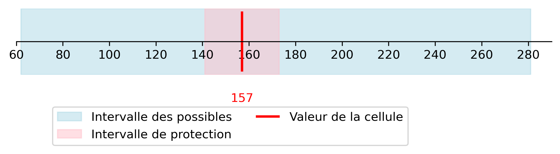
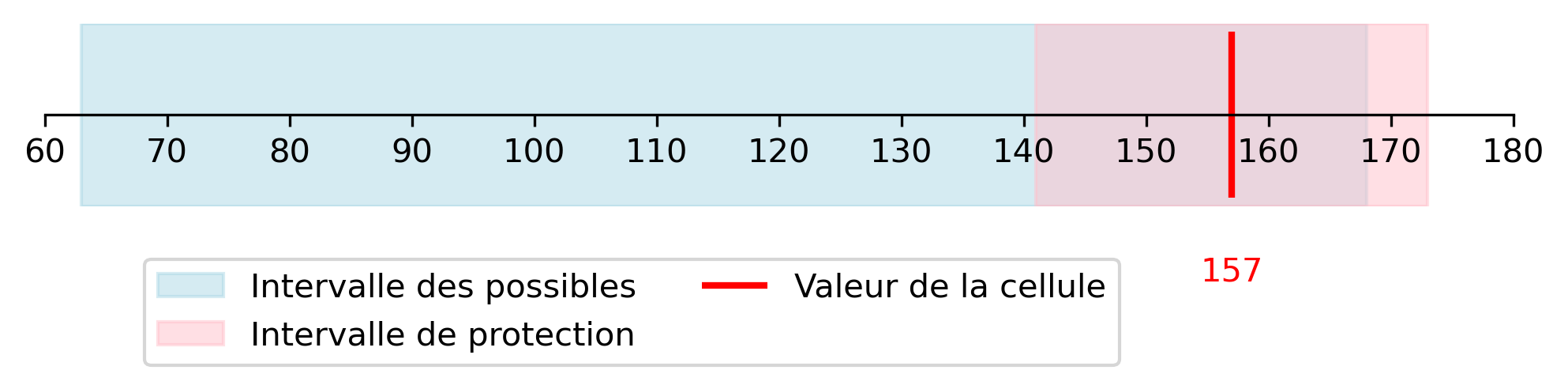
The upper bound of the interval of possibles (168) is lower than the upper bound of the protection interval (173).

Protection Intervals

We can infer the cell value at 7% and not 10%.

The cell is not sufficiently protected.

Protection Intervals

Another secret mask is used …

Region	Harp	Piano	Organ	Other	Total
North	58	X	X	800	1021
Center	11	X	X	934	1226
South	36	X	X	651	771
Total	105	219	309	2385	3018

Protection Intervals

… with other possible intervals.

Region	Harp	Piano	Organ	Other	Total
North	58	[0;163]	[0;163]	800	1021
Center	11	[0;219]	[62;281]	934	1226
South	36	[0;84]	[0;84]	651	771
Total	105	219	309	2385	3018

Protection Intervals

With this other secret mask, the cell is sufficiently protected.

Minimize Information Loss

To minimize information loss, it is necessary to define a cost associated with the suppression of each cell.

Several possibilities:

• The number of cells deleted
• The number of contributors affected by the deleted cells
• The value of the cell (default Tau-Argus)
• Another variable / adjusted cost

The Tools

\(\tau\)-Argus

• Allows calculation of primary and secondary suppression or controlled rounding
• Development, maintenance, and support: group of European experts coordinated by CBS
• Reference software in Europe for managing table confidentiality
• Free and open source software
• Latest stable version 4.2.4 (April 26, 2023)

\(\tau\)-Argus

👍	👎
Reference tool.	Cluttered interface.
High-performing on secret placement thanks to global optimization.	Bugs and errors not easy to understand and fix.
Tool regularly maintained.	Limited reproducibility of operations.

rtauargus

An R package to benefit from the advantages of \(\tau\)-Argus while limiting the drawbacks.

• Developed at Insee
• Open-source code
• Most recent version 06/25: v-1.3.0
• Online documentation
• Use the tab_XXX() functions

rtauargus

Package functionality:

• creates all the files in the formats expected by \(\tau\)-Argus
• Launches \(\tau\)-Argus
• Retrieves the results in R

rtauargus

1. Set the primary confidentiality “manually”
2. Set the secondary confidentiality with:

• tab_rtauargus(): to protect a single table
• tab_multi_manager(): to protect multiple tables

rtauargus

User feedback needed: create an issue on GitHub.

Or contact us by .

Hierarchies

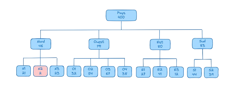
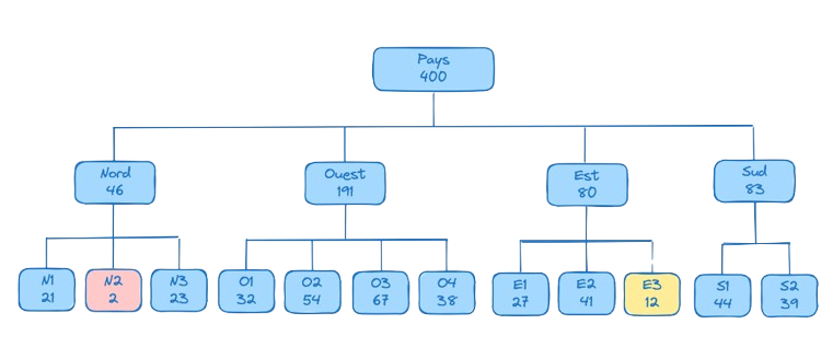
Hierarchical Tables

Hierarchical Tables

If the hierarchy is not specified, the hidden value can be retrieved.

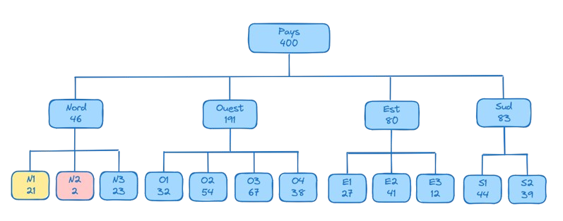
Hierarchical Tables

When the hierarchy is specified, the data is well protected.

The Argus format for hierarchies

In \(\tau\)-Argus hierarchies are presented in a specific format: .hrc text file.

• Must perfectly describe the nesting
• The number of @ designates the nesting level of each category
• Does not display the total
• The write_hrc2() function allows creating a .hrc file from a correspondence table

Protecting linked tables

Protecting Linked Tables with rtauargus

Use the tab_multi_manager() function:

1. The user describes the tables
2. Automatic merging of all tables with each other
3. Algorithm manages the iterative protection of the tables

N.B. The imposition of secrecy at each iteration is performed with \(\tau\)-Argus.

The tab_multi_manager() function provides a log in the form of reporting (secrecy imposition steps).

Analyze a Request

Analysis of a Request

It is necessary to identify the links between the tables to establish a secret that truly protects them.

The tables that are disseminated are not the same as the tables to be protected.

Steps of the analysis

1. Gather the information necessary for describing the tables

• field
• crosstabulation variables
• response variable (i.e. indicator)
• frequency or volume tables?
• description of nestings for hierarchies
• equations or correlations between response variables

Steps of the Analysis

2. Can the request be broken down into independent sub-requests?

• different fields and non-complementary \(\perp\!\!\!\perp\)
• different response variables (and not linked by an equation / correlation) \(\perp\!\!\!\perp\)
• all different crossover variables \(\perp\!\!\!\perp\)

In cases of independence, it is necessary to manage the different sub-requests separately.

Steps of the Analysis

3. List the tables necessary for applying the secret

• Certain hierarchies may lead to unifying tables
• If additive tables, construct a single table by creating an additional variable
• If non-nested hierarchy, extract the relevant levels to construct an additional table

Analysis Steps

4. Prepare the hierarchies

• Detect hierarchical variables
• Build the necessary .hrc files (manually or with write_hrc2())

Specific Links

Handling an Additive Relationship Between Response Variables

	reg1	reg2	T
tr1	5	10	15
tr2	12	18	30
tr3	5	5	10
T	22	33	55

Revenue knives

	reg1	reg2	T
tr1	3	8	11
tr2	6	20	26
tr3	2	6	8
T	11	34	45

Revenue forks

	reg1	reg2	T
tr1	8	18	26
tr2	18	38	56
tr3	7	11	18
T	33	67	100

Revenue flatware

Relationship between revenues: “flatware = knives + forks”.

Handling an additive link between response variables

New crossover variable: “type_couverts”.

Region	Tr	type_couverts	turnover
reg1	tr1	knives	5
reg1	tr1	forks	3
reg1	tr1	cutlery	8
…	…	…	…
Total	Total	cutlery	100

Handling a Non-Nested Hierarchy

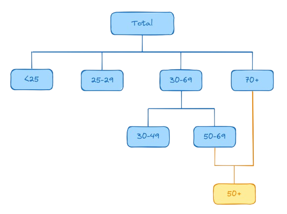
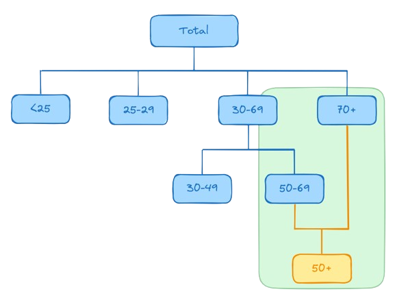
Here, the aggregate 50+ cannot be properly nested within the hierarchy.

Processing a non-nested hierarchy

Create a second table containing only the breakdown of 50+.

Handling a Non-Nested Hierarchy

princ.hrc

<25
25-29
30-69
@30-49
@50-69
70+

alt.hrc

50-69
70+

Create the Practical Guide

Protecting Tables with a Suppressive Method