Perturbative methods

For tabular data or microdata

INSEE, Department of Statistical Methods

Introduction

Objectives

  • What are the perturbative methods that allow limiting disclosure risks?
  • Which methods apply to tabular data, and which to individual data?
  • What type of risk do the methods protect us from?
  • What are the consequences on information loss?

Main methods available

Methods
Treatments Non-Perturbative Perturbative

Before tabulation
(on micro-data)
Resampling Noise injection
Variable recoding Micro-aggregation
Local suppression Swapping (rank or targeted)

After tabulation
(on aggregated data)
Variable recoding Rounding
Cell suppression Random keys
Differential privacy algorithm
Table 1: : Methods for managing data protection

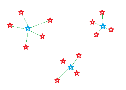
There is also another technique consisting of producing synthetic data.
Perturbative vs. Suppressive

In which cases should perturbative methods be preferred over suppressive methods?

  • Handling complex disseminations that are difficult to treat with suppressive methods:
    • numerous tables (industrial dissemination),
    • dissemination at multiple moments
    • geographic or nomenclature differentiation
  • Controlling the loss of utility more finely:
    • a possible trade-off in general by adjusting the noise parameters
    • no suppression => information available and manipulable
  • An institutional framework that authorizes such use

Perturbative vs. Suppressive

Some limitations of perturbative methods:

  • In some cases, loss of basic data characteristics (additivity in tables)
  • A less immediate perception of secrecy handling compared to blanking
  • Necessary education for the public regarding data usage
  • Historical secrecy rules to revisit, as they are adapted for suppressive methods

1 Post-Tabulation Methods

Post-tabulation methods

  • Methods that are applied to aggregated data
  • Some methods (particularly rounding) are more suitable for counts than for volumes
  • Perturbation of all or part of the tables according to the method

Some Challenges?

When perturbing data in tables:

  • Should everything be perturbed or only part of it?
  • How to ensure coherence between tables?
  • Should additivity be preserved within tables?

By answering these questions, one will orient towards one method rather than another.

An example

Suppose the following counting table (sensitive information in bold)

Characteristic North West South East Total
Polluting 6 14 1 7 28
Non-Polluting 3 2 1 13 19
Total 9 16 2 20 47
Table 2: Number of companies according to their location and the polluting nature of their activities

Deterministic or Random Rounding

Rounding

Rounding a count \(x\) means bringing its value to a multiple of the chosen rounding base \(b\):

  • Either to the nearest multiple (deterministic rounding)
    • => A deterministic rounding always returns the same value
  • Or, randomly, to one of the two nearest multiples (random rounding).
    • The rounding is unbiased by choosing the appropriate probabilities.
    • This technique offers better protection

Example

\(b=10\) and \(x=23\):

  • Deterministic rounding: \(x^\prime = 20\).
  • Random rounding:
    • \(x^\prime = 20\) with probability of \(0.7\) or
    • \(x^\prime = 30\) probability of \(0.3\).

An example

Characteristic North West South East Total
Polluting 5 15 0 5 30
Non-Polluting 5 0 0 15 20
Total 10 15 0 20 45
Table 3: Application of a deterministic base rounding \(b=5\) (Average of absolute deviations: \(1.4\).)

Rounding of Small Counts

Small Count Rounding

Algorithm applied to data tables ensuring:

  • rounding of small counts (i.e., the most sensitive ones) in a base \(b\)
  • additional counts are adjusted to:
    • preserve additivity in the tables
    • and minimize the overall perturbation

Technique implemented in the R package SmallCountRounding

An Example

Characteristic North West South East Total
Polluting 6 14 0 7 28
Non-Polluting 5 0 0 13 18
Total 11 14 0 20 45
Table 4: Application of a Small Count Rounding type algorithm (Mean absolute deviation: \(1.07\).)

Controlled Rounding

Controlled Rounding

Algorithm applied to data tables ensuring:

  • rounding of all counts to a base \(b\)
  • while ensuring:
    • preservation of additivity in the tables
    • minimization of the sum of absolute differences between original and rounded values

Technique implemented in the software Tau-ARGUS

An example

Characteristic North West South East Total
Polluting 5 15 0 5 25
Non-Polluting 5 2 0 15 20
Total 10 15 0 20 45
Table 5: Application of controlled rounding with a base \(b=5\) (Average of absolute deviations: \(1.5\).)

3 The random keys method (CKM)

The Random Keys Method

A method that consists of deviating all counts independently from one another:

  • each count is deviated by a value between \(-D\) and \(+D\), where \(D\) is a parameter of the method;
  • a cell is always perturbed in the same way through the use of individual keys
  • a null count is not perturbed;
  • the amount of noise injected into the tables has variance \(V\), another parameter of the method.

Sources: Thompson et al. (2013), Chipperfield et al. (2016), Gießing and Tent (2019)

Probability Distribution

Properties:

  • A maximum deviation D and a variance V are fixed upstream

  • The injected noise is unbiased

  • The probability law of the injected deviation is defined from a transition matrix

An example

Characteristic North West South East Total
Polluting 4 15 0 8 28
Non-Polluting 1 3 2 15 20
Total 10 16 4 21 46
Table 6: Application of the CKM with \(D = 5\) and \(V = 3\) (Average of absolute deviations: \(1.1\))

Uses

The method is used by several NSIs:

  • Since 2006, ABS has provided an online querying tool to obtain data from its quinquennial census. The data is protected with the CKM. (https://tablebuilder.abs.gov.au)

  • The CKM is one of the methods recommended by Eurostat to protect the 2021 European Census data.

  • In this context, Destatis uses the CKM to disseminate data on 500m grids.

  • 2024/2025: the Insee disseminates data on the Neighborhoods of the City Policy (QPV).

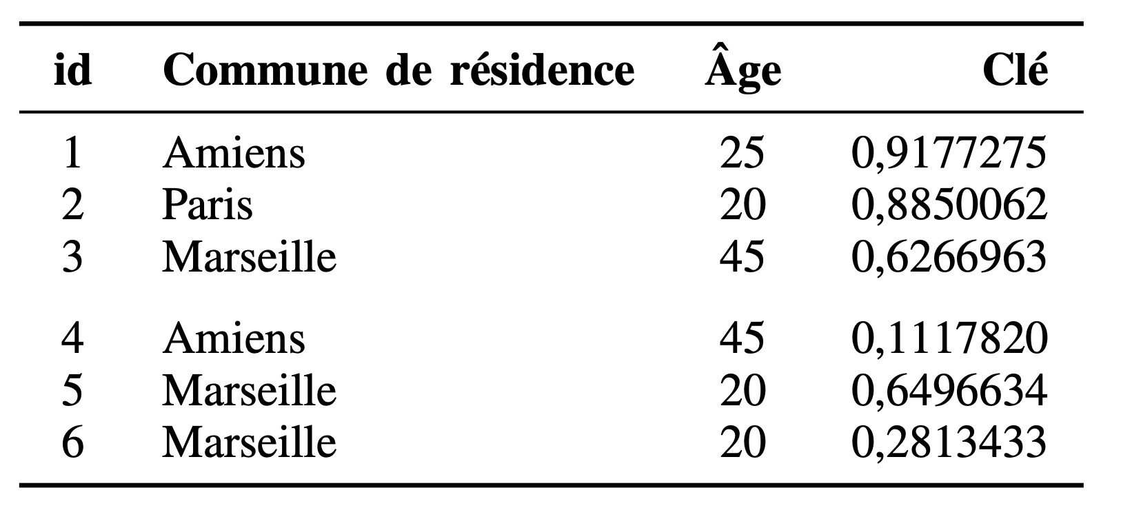
Step 1: Creation of a Random Individual Key

Ajout des clés individuelles aux micro-données
Figure 1: Arbitrer

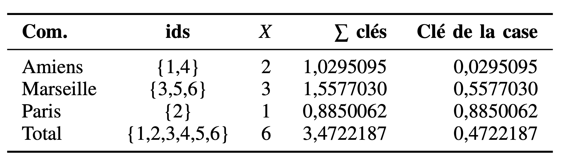
Step 2: Construction of the table

Construction of the table and the keys for each cell
Figure 2: Construction of the table and the keys for each cell

Step 3: Transition Probabilities

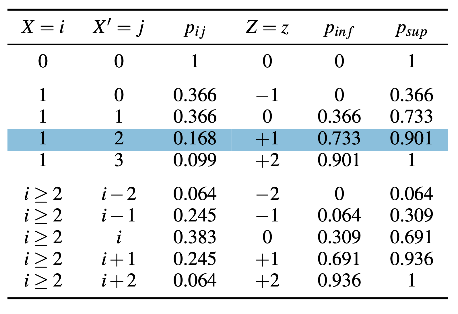
Transition matrix for D=2 and V=1
Figure 3: Transition matrix for D=2 and V=1

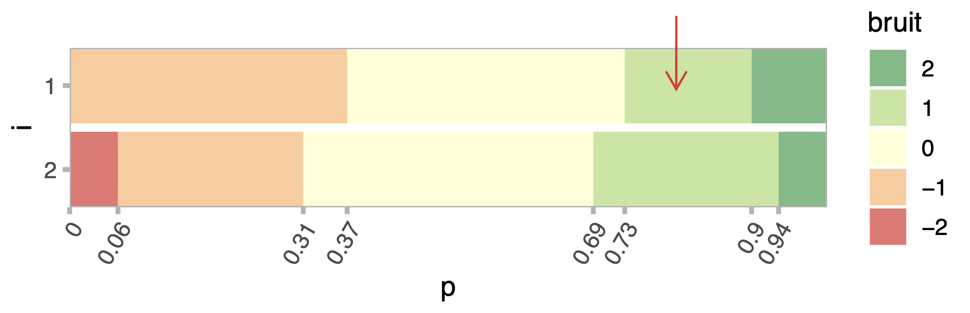
Step 4: Determine the perturbation to inject

The perturbation to inject
Figure 4: The perturbation to inject” fig-align=“center

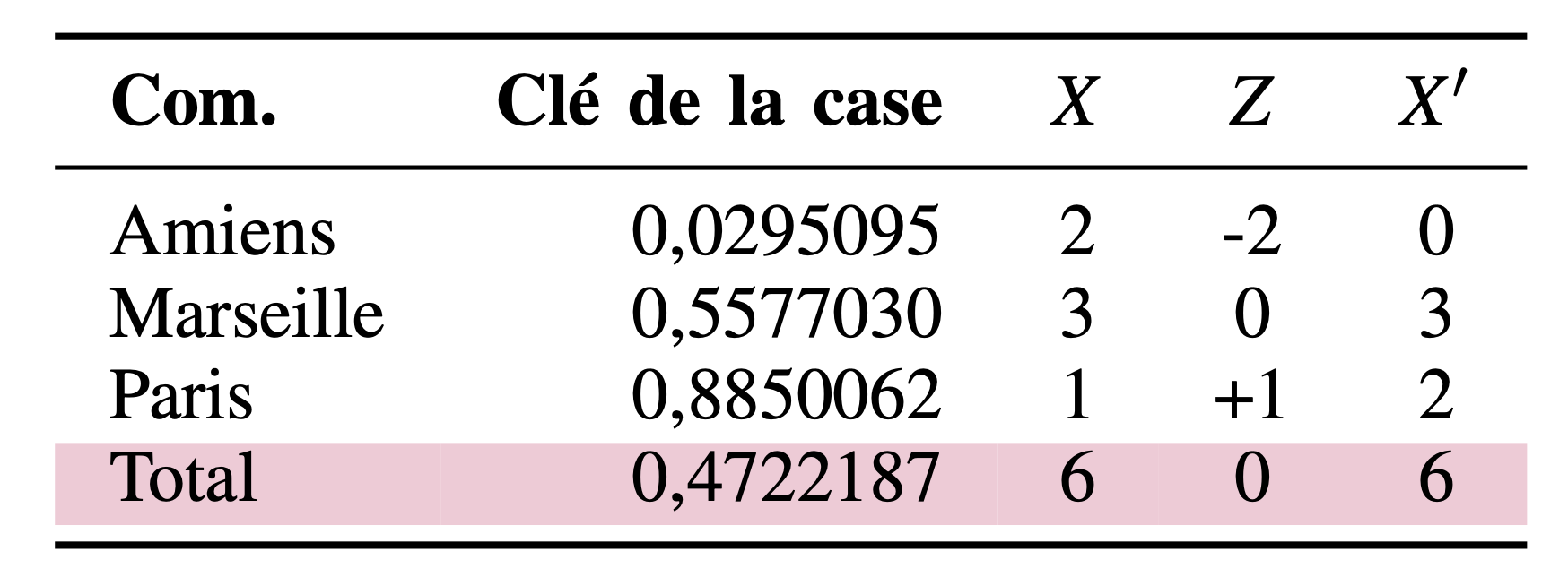
Step 5: Build the final table

Table after perturbation
Figure 5: Table after perturbation

Advantages / Disadvantages

Advantages Disadvantages
Easy to implement Loss of additivity
Table consistency Perception of secret management less straightforward
Reduces differentiation risks Accumulation of noise for second-order statistics (ratios for example)
Compatible with querying
Compatible with custom dissemination
Better utility than rounding at equal protection level
Table 7: Advantages and disadvantages of the random key method

4 Microaggregation

  • Perturbative method, more suited to continuous variables, but may be adapted to ordered categorical variables

  • Main idea:

    • Create small homogeneous groups by taking into account the values of selected variables

    • Replace the values of all individuals belonging to the group with a single value (may be the average value of values observed in the group)

An Example

Region Age Hours Worked per Week Monthly Income
92 36 17 1000
75 41 35 2000
75 52 0 1100
94 45 35 2500
75 41 0 1900
92 26 46 1500
92 31 38 800
94 48 30 1200
Table 8: Individual data with unique observations on Age \(\times\) Region intersections

An example

Region Age Hours worked per week Monthly income
92 36 31 17 1000
75 41 45 35 2000
75 52 45 0 1100
94 45 47 35 2500
75 41 45 0 1900
92 26 31 46 1500
92 31 31 38 800
94 48 47 30 1200
Table 9: Individual data with uniques on the Age \(\times\) Region crossings
  • \(\mu_{red} = 45\), \(\mu_{yellow} = 31\), \(\mu_{green} = 47\)

Parameters

A large number of possible outputs for this method depending on:

  • the chosen definition of homogeneity

  • the algorithm used to build the groups

  • the determination of the replacement value

The parameters to define:

  • Size \(g\) of each group (the larger the group size, the greater the loss of information, and the larger it is, the higher the level of protection ..)

  • Which variables are used to calculate the distance?

  • Which statistics to choose once the groups have been formed? (mean, median?)

Minimize within-group variance

Minimization of within-group variance
Figure 6: Table after perturbation

The algorithm seeks to minimize the sum of within-group squared errors:

\[SSE = \sum_{i=1}^g\sum_{j \in i} (x_{ij}-\bar x_{i})^T(x_{ij}-\bar x_{i})\]

Advantages / Disadvantages

Advantages Disadvantages
Suitable for \(k\)-anonymity High computation time
Statistically relevant classes
Table 10: Advantages and disadvantages of injecting additive noise

5 Additive Noise Injection

Noise Injection

  • Method adapted for handling continuous variables

  • In general, an unbiased additive noise with fixed variance is injected

  • Main challenge: how to add noise while preserving the characteristics of the variables and any potential relationships between them?

Perturbation by Additive Noise

  • Noise is added to each observed value
  • Generally zero-mean Gaussian noise
  • Suitable for continuous variables of low amplitude

Independent Additive Noises

  • Each variable is noised independently of the other variables

  • The means and covariances of each perturbed variable are preserved

  • But, the variances and the correlation coefficients are not preserved

Correlated Additive Noise

  • The variance-covariance matrix of the noise is proportional to the variance-covariance matrix of the original values

  • Preservation of the mean and correlation coefficients

  • Preferable to adding independent noise because unbiased estimates can be obtained for several important statistics

Advantages / Disadvantages

Advantages Disadvantages
Processing of sensitive continuous variables Not suitable for handling outliers with large values
Preservation of important statistics
Table 11: Advantages and disadvantages of additive noise injection

6 Targeted Record Swapping (TRS)

Targeted Record Swapping (TRS)

Definition

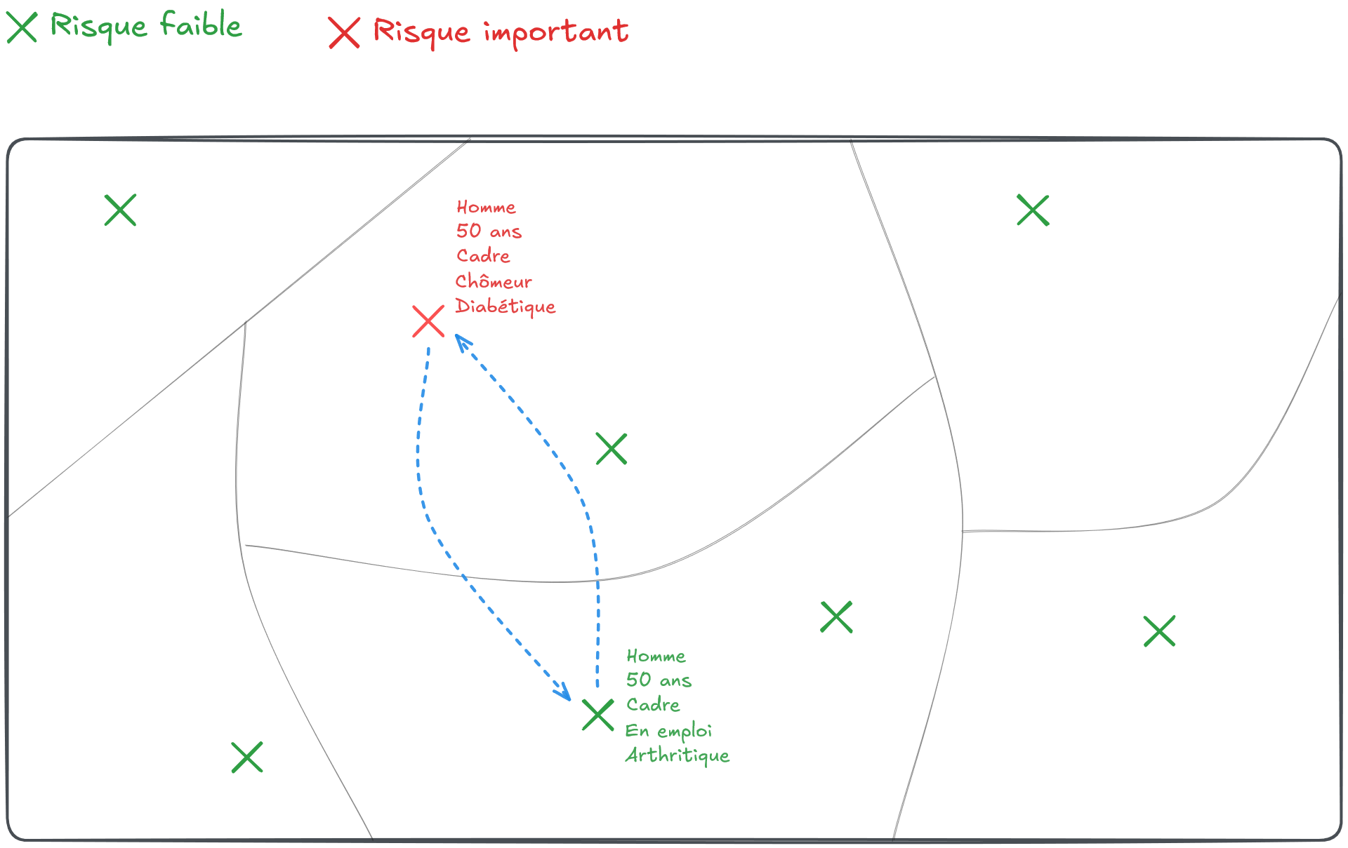
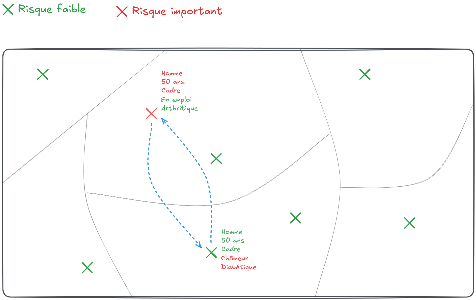
Target Record Swapping (TRS) is a method applied directly to an individual dataset to reduce re-identification risks.

It consists of swapping the location of certain individuals deemed at risk with other individuals from another geographic entity.

Hence its name: swapping, that is, the exchange, will concern units from the database (the records) detected in advance, thus becoming the targets on which the exchange will focus.

At-risk individuals (targets)

  • Targets at-risk individuals:
    • Detection by \(k\)-anonymity: crossings of quasi-identifiers of fewer than \(k\) individuals
    • Detection by \(l\)-diversity: homogeneity of a group on a sensitive variable
    • Probabilistic measure of individual risk
    • Primarily a risk of re-identification

A very widely used method

  • Insee: European census 2021 data

  • Eurostat recommends this method (coupled with CKM) for disseminating the European Census

  • US Census Bureau: US Census 2010

  • ONS (UK): Census since 2010

An example

Before swapping
Figure 7: Before Swapping

An Example

After swapping
Figure 8: After Swapping

Advantages / Disadvantages

Advantages Disadvantages
Effective for handling different types of risk Requires setting a large number of parameters (risk measure, similarity variables, swapping rate)
Flexible method, adaptable to very different cases (household-individual structures for example) Noise injected into the data is not really controllable
Preserves aggregates at the geographic level within which swapping was performed. Generates local bias in the data
Maintains additivity of tables generated from noisy micro-data.
Table 12: Advantages and disadvantages of TRS

7 Post-Randomisation Method (PRAM)

PRAM Method

  • Allows processing sensitive categorical variables by adding noise to the data.

  • Consists of randomly modifying the assignment of individuals to a given class.

  • Method particularly useful for handling disclosures of sensitive attributes: an attacker cannot have any certainty about the attribute of an observation.

An example

Region Age Professional situation
92 14 Inactive
75 41 Unemployed
75 52 Active
94 45 Active
75 41 Unemployed
92 26 Active
92 31 Active
94 14 Inactive
  • Inactive: 2 ind., Unemployed = 2 ind., Active = 4 ind.

An example

Region Age Employment Status Employment Status (PRAM)
92 14 Inactive Unemployed
75 41 Unemployed Employed
75 52 Employed Employed
94 45 Employed Employed
75 41 Unemployed Inactive
92 26 Employed Employed
92 31 Employed Unemployed
94 48 Inactive Inactive
  • Inactive: 2 ind., Unemployed = 2 ind., Employed = 4 ind.

An example

Region Age Pro. situation Pro. situation (PRAM)
92 14 Inactive Unemployed
75 41 Unemployed Active
75 52 Active Active
94 45 Active Active
75 41 Unemployed Inactive
92 26 Active Active
92 31 Active Unemployed
94 48 Inactive Inactive
  • Watch out for inconsistencies!

The transition matrix

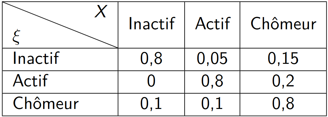
We need to define a transition matrix to specify the transition probabilities.

  • Let \(\xi\) be the initial categorical variable with \(K\) categories \(1 \dots K\)
    \(\rightarrow\) in the example, \(\xi\) = Professional situation, K = 3

  • Let \(X\) be the same categorical variable in the perturbed dataset
    \(\rightarrow\) in the example, \(X\) = Professional situation (PRAM) ## The transition matrix We can define the transition matrix \(P\),

\[P =(p_{kl})_{1 \leq k,l \leq K}\]

where \(p_{kl} = P(X =l|\xi = k)\)

How to Choose the Transition Matrix?

  • PRAM randomly changes the population counts:

    \[\mathbb{E}\begin{pmatrix} N^{pram}_{I} \\N^{pram}_{E}\\ N^{pram}_{U} \end{pmatrix} = P^{T} \begin{pmatrix}N_{I} \\N_{E}\\ N_{U} \end{pmatrix}\]

  • Depending on P and the original counts, the margins can be greatly disturbed!

  • High diagonal coefficients may be insufficient

A Numerical Example

  • Original Margins

    Ina ctive Ac tive U nemployed
    Frequency (million) 16.8 49 4.2
    Percentage 24 % 70 % 6 %
  • Transition Matrix \(P\) :

A numerical example

We can now calculate the perturbed margins!

  • Original margins

    Status Inactive Active Unemployed
    Frequency (million) 17 49 4
    Percentage 24% 70% 6%
  • New margins

    Status Inactive Active Unemployed
    Frequency 14 41 16
    Percentage 20% 58% 22 %

PRAM Invariant

  • Possibility of choosing the matrix \(P\) such that the perturbation is unbiased \(\rightarrow\) PRAM invariant

  • Given that : \[\mathbb{E}\begin{pmatrix} N^{pram}_{I} \\N^{pram}_{E}\\ N^{pram}_{U} \end{pmatrix} = P^{T} \begin{pmatrix}N_{I} \\N_{E}\\ N_{U} \end{pmatrix}\]

  • For this, it is necessary to choose \(P\) such that the original marginal frequencies are an eigenvector of \(P\) associated with the eigenvalue \(1\).

Measuring the level of protection

  • PRAM deliberately introduces a measurement error \(\rightarrow\) k-anonymity or l-diversity cannot be used

  • Level of protection measured from the method’s parameters (transition matrix).

  • Idea: make the rarity of certain modalities sufficiently uncertain to infer \(\rightarrow\) posterior odds ratio

Measuring the level of protection

\[POST\_ODDS(k) = \frac{P(\xi = k|X=k)}{P(\xi \neq k|X=k)} = \frac{p_{kk}P(\xi = k)}{\sum_{l \neq k}p_{lk}P(\xi=l)}\]

  • \(p_{kk}\) are known and depend on the sampling design
  • \(P(\xi = k)\) can be difficult to estimate
  • we can roughly estimate \(P(\xi = k)\) by \(\frac{T_\xi(k)}{n}\)

Interpretation

We observe k in the perturbed game:

  • If \(POST\_ODDS(k) > 1\), then the original value is more likely \(k\) rather than another value.

  • If \(POST\_ODDS(k) < 1\), then the original value is more likely another value than \(k\).

Advantages / Disadvantages

Advantages Disadvantages
Allows providing the level of protection associated with injected noise by calculating inverse transition probabilities Creation of potentially impossible combinations (e.g., retired child).
Preserves the additivity of tables generated from noisy microdata. Difficult to define a protection matrix that accounts for relationships with all variables.
Table 13: Advantages and disadvantages of PRAM

8 Synthetic Data

  • Idea: Generate all or part of individual data.

  • Two types of synthesis:

    • Complete synthesis: all variables and all individuals are generated.

    • Partial synthesis: Only certain variables are generated (mainly sensitive variables).

Sequential Modeling

Fully Conditional Specification

Each variable in the dataset is modeled sequentially and conditionally on the previous variables.

To generate the \(p^e\) variable, we seek to model its conditional distribution:

\[f_{X_p | X_1 , X_2 , \dots , X_{p-1}}\]

Commonly used statistical models: - parametric models (linear or logistic regression) - tree-based methods: CART, Boosting, random forest, XGBoost.

Deep Learning Methods (I)

Tabular Variational Auto Encoder (TVAE)

Autoencoding consists of combining an encoding phase that reduces the dimension of the data to learn the most important features and a decoding phase to reconstruct data in their original dimension.

Deep Learning Methods (II)

Conditional Tabular Generative Adversarial Network (CTGAN)

GANs are very popular in image generation. CTGANs are an adaptation of GANs for generating tabular data (microdata or aggregated data). A generator constructs synthetic data and submits it to a discriminator whose objective is to distinguish this generated data from the original data.

References

Chipperfield, James, Daniel Gow, and Bronwyn Loong. 2016. “The Australian Bureau of Statistics and Releasing Frequency Tables via a Remote Server.” Statistical Journal of the IAOS 32 (1): 53–64. https://doi.org/10.3233/SJI-160969.
Gießing, Sarah, and Reinhard Tent. 2019. “Concepts for Generalising Tools Implementing the Cell Key Method to the Case of Continuous Variables.” UNECE - Expert Meeting on Statistical Data Confidentiality (the Hague), October. https://unece.org/fileadmin/DAM/stats/documents/ece/ces/ge.46/2019/mtg1/SDC2019_S2_Germany_Giessing_Tent_AD.pdf.
Hundepool, Anco, Josep Domingo-Ferre, Luisa Franconi, et al. 2024. Handbook on Statistical Disclosure Control. 2nd Edition. ESSNet SDC. https://sdctools.github.io/HandbookSDC/.
Thompson, Gwenda, Stephen Broadfoot, and Daniel Elazar. 2013. “Methodology for the Automatic Confidentialisation of Statistical Outputs from Remote Servers at the Australian Bureau of Statistics.” Joint UNECE/Eurostat Work Session on Statistical Data Confidentiality (Ottawa), October. https://unece.org/fileadmin/DAM/stats/documents/ece/ces/ge.46/2013/Topic_1_ABS.pdf.