Assessing Utility

Control the loss of information

INSEE, Department of Statistical Methods

1 Define

How to define it?

  • The data protection process necessarily leads to a loss of information
Region Age Status
92 14 Inactive
75 41 Unemployed
75 52 Employee
94 45 Employee
75 41 Unemployed
92 26 Employee
92 31 Employee
94 14 Inactive
Table 1: risk = 100 % , Info loss = 0 %
Region Age Status
∅ ∅ ∅
∅ ∅ ∅
∅ ∅ ∅
∅ ∅ ∅
∅ ∅ ∅
∅ ∅ ∅
∅ ∅ ∅
∅ ∅ ∅
Table 2: risk = 0 % , Info loss = 100 %

What uses for the data?

  • Depending on the end users, the concept of information loss can change

  • Know the uses that will be made of the data (e.g. regression, aggregates, averages)

  • It is not recommended to publish multiple protected versions of the same dataset for each type of user \(\rightarrow\) significant disclosure risks through differentiation.

Main idea

Two ways to measure information loss:

  1. Compare the raw records between the original dataset and the protected dataset

  2. Compare certain statistics calculated on the original and protected datasets

2 Continuous data

Notations

For continuous data, formally:

  • \(I_1,\dots, I_n\), \(n\) individual records

  • \(Z_1,..,Z_p\), \(p\) continuous variables

  • \(X\) the original data matrix, \(X^{'}\) the protected data matrix

Distance between matrices

  • Mean squared error: sum of the squared differences between the two matrices, component by component, divided by the number of coefficients in a matrix (same for both) \[\frac{1}{np}\sum_{j=1}^p\sum_{i=1}^n(x_{ij}-x^{'}_{ij})^2\]

Distance between matrices

  • Mean absolute error: sum of the absolute differences between the two matrices, component by component, divided by the number of coefficients in a matrix (same for both) \[\frac{1}{np}\sum_{j=1}^p\sum_{i=1}^n|x_{ij}-x^{'}_{ij}|\]

Distance between matrices

  • Mean variation: sum of the absolute variations in percentage of the components of the protected matrix relative to the original data matrix \[\frac{1}{np}\sum_{j=1}^p\sum_{i=1}^n\frac{|x_{ij}-x^{'}_{ij}|}{|x_{ij}|}\]

With \(x_{ij} \ne 0\).

“On average, each cell has been modified by x% compared to the original value.”

An example

Sex Reg Age h / week
F 92 36 17
M 75 41 35
F 75 52 5
Table 3: Hours worked per week by sex, age and region (original data \(X\))
Sex Reg Age h / week
F 92 34 23
F 75 48 35
M 75 58 2
Table 4: Hours worked per week by sex, age and region (perturbed data \(X^{'}\))

An example

  • Mean squared error =

\(\frac{(36-34)^2+(41-48)^2+(52-58)^2+(17-23)^2+(35-35)^2+(5-2)^2}{6}=22\)

  • Mean absolute error =

\(\frac{|36-34|+|41-48|+|52-58|+|17-23|+|35-35|+|5-2|}{6}=4\)

  • Mean variation =

\(\frac{\frac{|36-34|}{36}+\frac{|41-48|}{41}+\frac{|52-58|}{52}+\frac{|17-23|}{17}+\frac{|35-35|}{35}+\frac{|5-2|}{5}}{6}=0.15\)

Effect of size on mean variation

The mean variation depends on the size of \(x_{ij}\):

  • Large \(x_{ij}\) \(\rightarrow\) even a large difference \(|x_{ij} - x^{'}_{ij}|\) gives a low ratio

  • Small \(x_{ij}\) \(\rightarrow\) even a small absolute difference \(|x_{ij} - x^{'}_{ij}|\) gives a high ratio

Correcting the size effect

To make the ratio independent of the size of \(x_{ij}\), another measure is used: \[\frac{1}{np}\sum_{j=1}^p\sum_{i=1}^n\frac{|x_{ij}-x^{'}_{ij}|}{\sqrt{2}S_j}\] with \(S_j\) the standard deviation of the \(j\)-th variable

Allows comparing variations to the “normal” variability of the variable.

Specific measures

  • Univariate comparisons (comparison of a variable’s distribution before and after perturbation).

  • Bivariate comparisons: Linear correlations, for example.

  • Multivariate comparisons: Comparison of the planes of a principal component analysis.

  • Comparison of regression parameters, etc.

3 Categorical data

Different comparisons

For categorical variables, 3 main ideas to evaluate information loss with categorical data:

  • Direct comparison of variable values

    • Mean absolute differences

    • Mean relative absolute differences

  • Comparison of contingency tables

  • Measures based on entropy

Entropy-based measure

  • Entropy measures the uncertainty induced by a given probability distribution: \[H(V|V^\prime=j) = - \sum_{i=1}^K P(V=i|V^\prime = j) \log(P(V=i|V^\prime = j))\]

  • Depending on the method, it can be difficult to evaluate the quantity \(P(V=i|V^{'} = j)\)

  • Global risk \[R = \sum_{r \in enregistrements} H(V|V^\prime=\underset{protected value}{\underbrace{j_{r}}})\]

Measuring inference quality

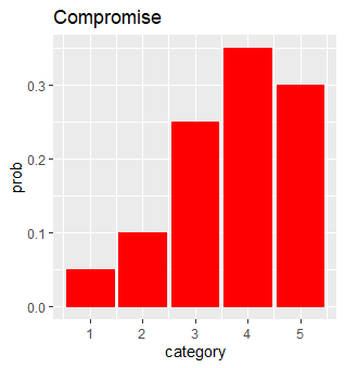
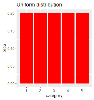
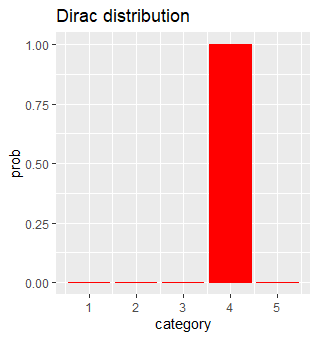
  • \(K = 5\) categories, say \(j = 4\), and examine \(P(V=i|V^{'} = 4)_{1\leq i\leq 5}\)
No noise
Figure 1: Dirac
Compromise
Figure 2: Compromis
Strong noise
Figure 3: Bruit fort
  • Trade-off between risk and information loss!

Global measures

  • Mean absolute or relative differences
  • Hellinger distance
    \[HD(\mathbf{X}, \mathbf{X}') = \frac{1}{\sqrt{2}} \sqrt{\sum_{j = 1}^M \left(\sqrt{\frac{x'_j}{\sum_{j=1}^M x'_j}} - \sqrt{\frac{x_j}{\sum_{j=1}^M x_j}}\right)^2}\]

Specific metrics for contingency tables

  • Comparison of Cramer’s V (based on the \(\chi^2\) statistic)
  • Comparison of the first factorial plane of a correspondence analysis.

4 Rely on visualization

Many possibilities

  • Univariate: histograms, box plots, bar charts
  • Bivariate: Correlation matrices, mosaic plots, Plane of a correspondence analysis, etc.
  • Multivariate: 1st plane of a factorial analysis (PCA, MCA, MFA)

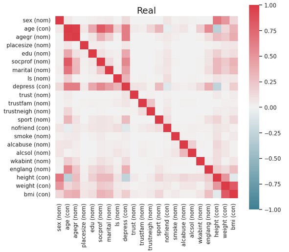
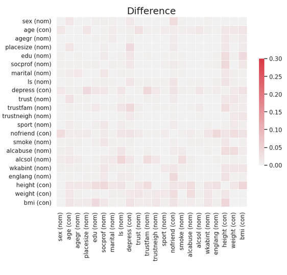
Correlation matrix

Original correlation matrix
Figure 4: Original
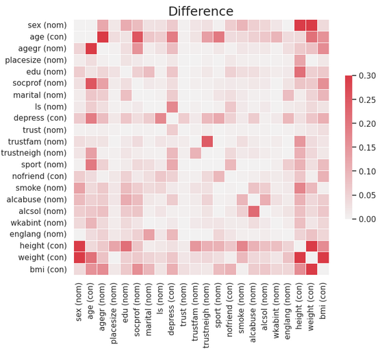
Matrix of differences between original and method 1
Figure 5: Differences method 1
Matrix of differences between original and method 2
Figure 6: Differences method 2

Visual comparison immediately shows that the first method preserves bivariate relationships better than the second.

Clouds from a factorial analysis

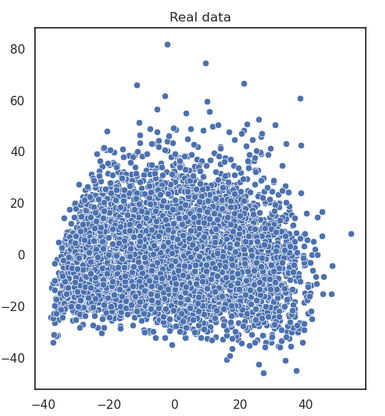
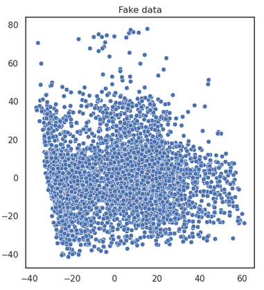
Comparison of the projection of individuals on the first plane of a factorial analysis.
Original individuals projected on the first plane of a PCA
Figure 7: Original
Noisy individuals projected on the first plane of the same PCA
Figure 8: Perturbed

Results of a regression

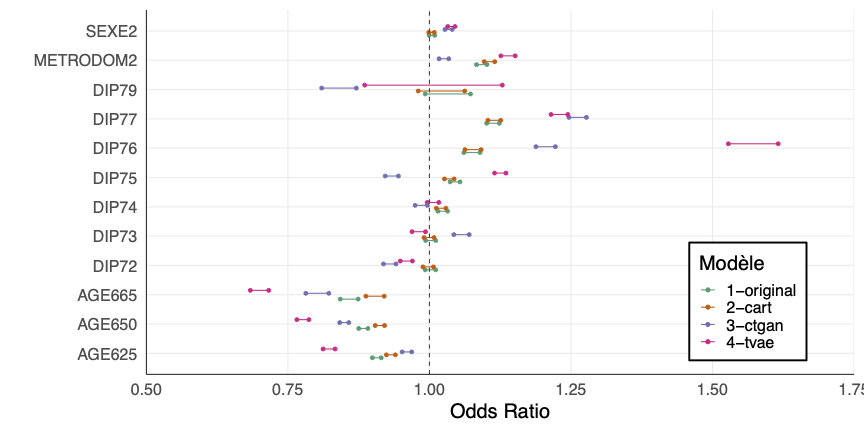
Confidence intervals of logistic regression coefficients depending on the data processing method
Figure 9: Confidence interval of logistic regression coefficients according to the data processing method