Risk profile as a function of dominance

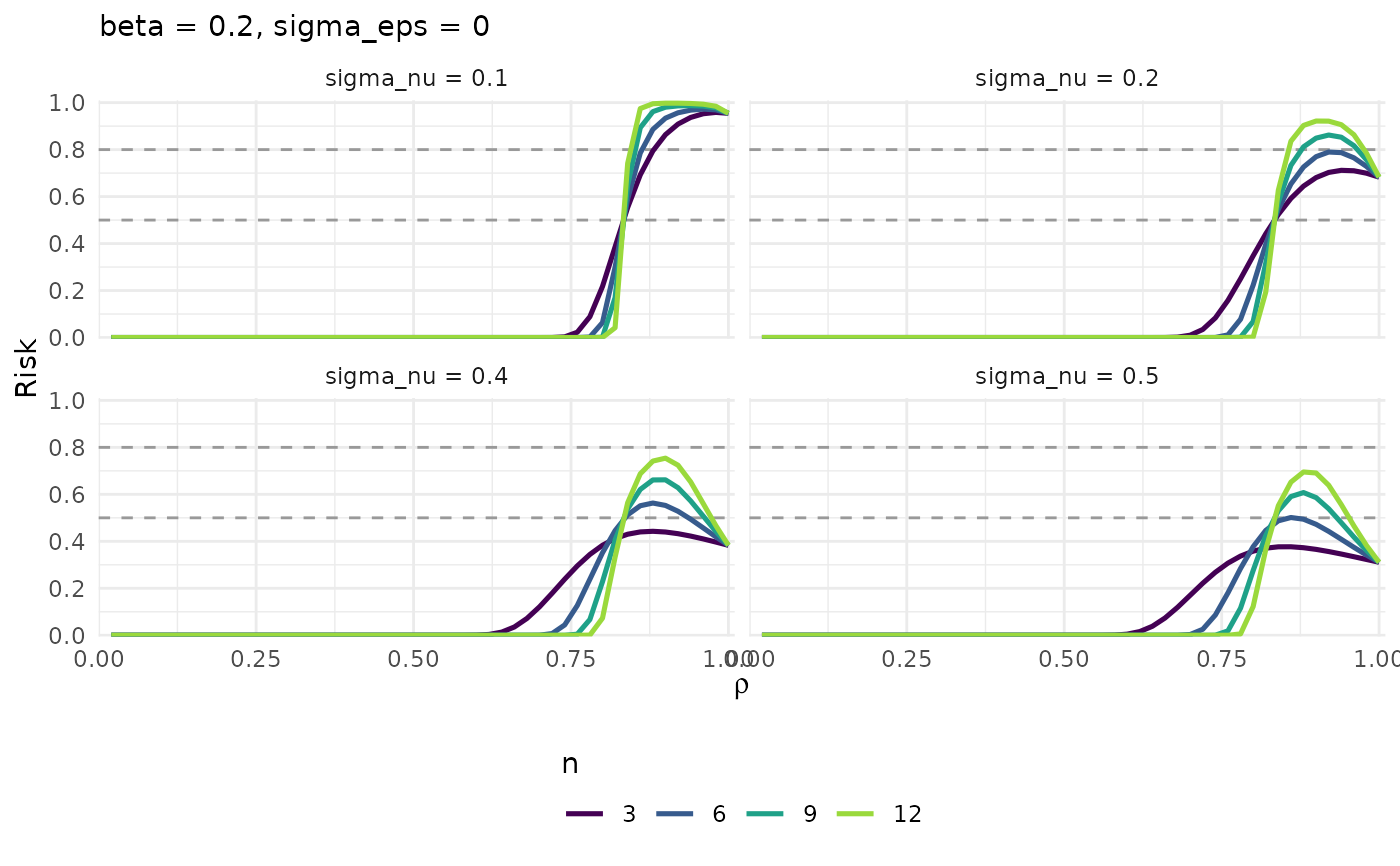
Reproduces Figure 2 of the paper, generalised: the disclosure risk against the dominance level rho, one curve per shape parameter n, panels split by sigma_nu (and by scenario when the table carries several).

Usage

pm_plot_risk_profile(
  x,
  sigma_nu = NULL,
  n = NULL,
  beta = NULL,
  sigma_eps = NULL,
  scenario = NULL,
  thresholds = c(0.5, 0.8)
)

Arguments

x

A calibration table (e.g. from pm_calib_dominance()).

sigma_nu, n, beta, sigma_eps, scenario

Optional values to keep; NULL keeps everything present in the table. Filtering is usually needed on beta and sigma_eps to keep the panel grid readable.

thresholds

Risk levels drawn as dashed horizontal lines.

Value

A ggplot object.

Examples

grid <- pm_calib_dominance(beta = c(0.1,0.2))
pm_plot_risk_profile(grid, sigma_nu = c(0.1, 0.2, 0.4, 0.5), beta = 0.2)