Worst-case risk against a mechanism parameter

Reduces a calibration table to the worst case over rho of the disclosure risk, at a fixed sigma_eps, and plots it against one of the two mechanism parameters. Panels are split by scenario when several are present.

Usage

pm_plot_risk_max(
  x,
  x_axis = c("sigma_nu", "n"),
  sigma_nu = NULL,
  n = NULL,
  beta = NULL,
  sigma_eps = NULL,
  scenario = NULL,
  tau = NULL,
  mark_frontier = NULL,
  marks = NULL,
  thresholds = c(0.5, 0.8)
)

Arguments

x

A calibration table (e.g. from pm_calib_dominance()). Needs a fine grid on the x-axis parameter to draw smooth curves.

x_axis

Parameter on the x-axis: "sigma_nu" (default) or "n".

sigma_nu, n, beta, sigma_eps, scenario

Optional values to keep; NULL keeps everything present in the table.

tau

Optional risk ceiling, drawn as an extra dashed line on top of thresholds. A single value is required to mark the frontier.

mark_frontier

Whether to mark the largest admissible n of each sigma_nu. NULL (default) marks it whenever it is defined, i.e. when x_axis = "n" and a single tau is given. TRUE forces it and warns when it cannot be drawn; FALSE never draws it.

marks

Values of the x-axis parameter highlighted with a point; NULL (default) for none.

thresholds

Risk levels drawn as dashed horizontal lines.

Value

A ggplot object.

Details

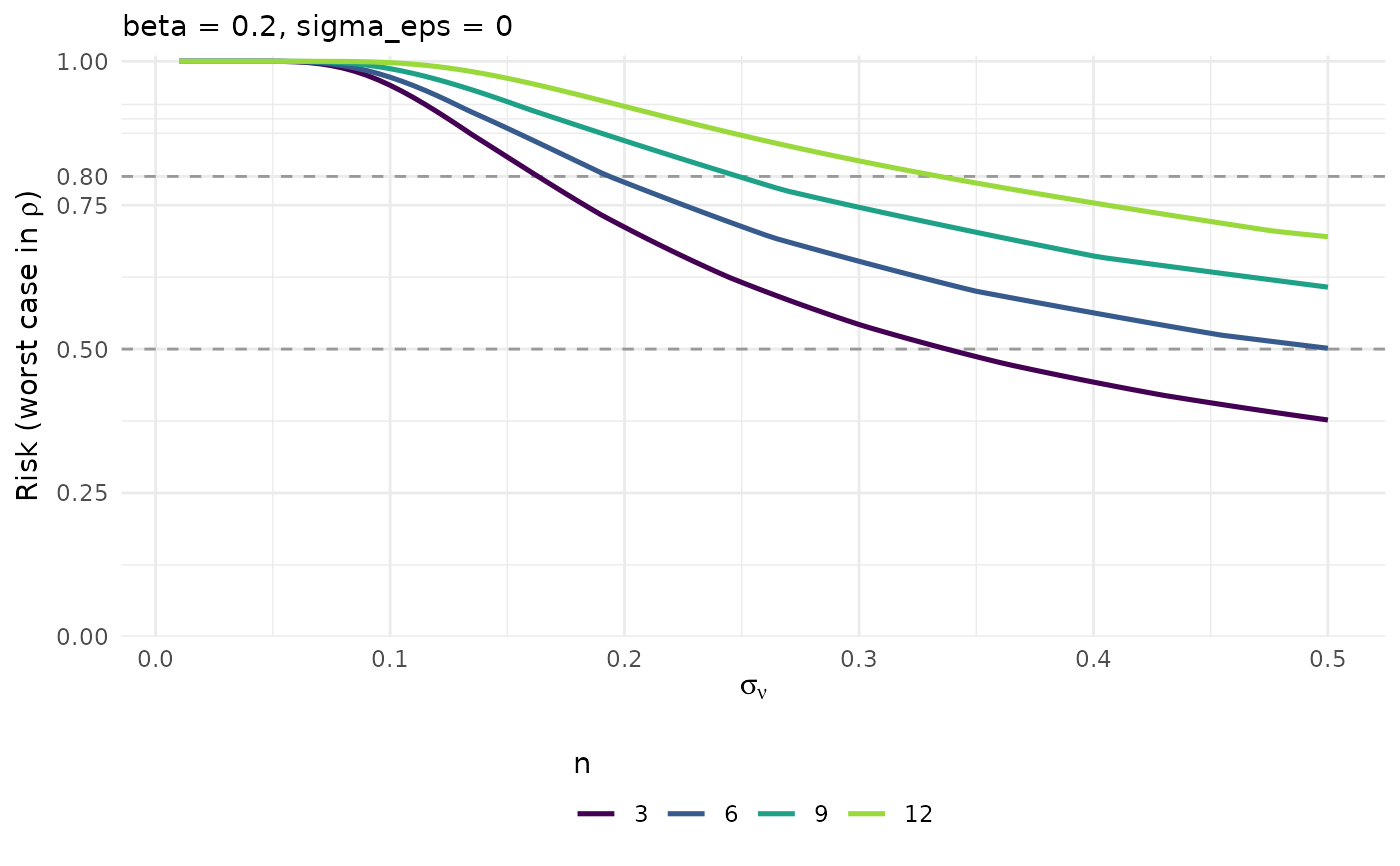
With x_axis = "sigma_nu" (default) this reproduces the middle panel of Figure 3 of the paper, generalised: the risk decreases with sigma_nu, one curve per n.

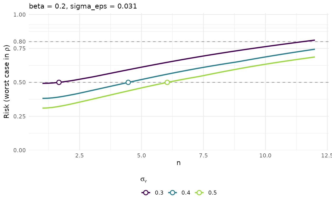
With x_axis = "n" it is the view that accompanies pm_suggest_n(): the risk increases monotonically with n, one curve per sigma_nu. Each crossing of the ceiling tau is the n_max of its sigma_nu – the very root that pm_suggest_n() solves for. Those points are overlaid when mark_frontier allows it, computed by the same function so that the plot and the table always agree.

See also

pm_suggest_n(), plot.pm_calib_dominance().

Examples

# Figure 3 (middle panel): worst-case risk against sigma_nu
grid <- pm_calib_dominance(sigma_nu = (2:100)/200,
                           n = c(3, 6, 9, 12), beta = 0.2)
pm_plot_risk_max(grid, marks = c(0.05, 0.1, 0.2, 0.3, 0.4, 0.5))


# Against n, with the frontier found by pm_suggest_n()
grid <- pm_calib_dominance(sigma_eps = 0.031, beta = 0.2,
                           sigma_nu = c(0.3, 0.4, 0.5), n = (5:60)/5)
pm_plot_risk_max(grid, x_axis = "n", tau = 0.5)